Usage
Basic Usage
This page provides a comprehensive guide on how to use dustysn to fit SEDs of supernovae using different dust emission models.
The most basic function is calc_model_flux, which generates a model dust emission spectrum.
from dustysn.model import calc_model_flux
from astropy import units as u
import numpy as np
import matplotlib.pyplot as plt
plt.rcParams.update({'font.size': 12})
plt.rcParams.update({'font.family': 'serif'})

# Basic parameters
dust_mass = 0.0008  # Solar masses
temperature = 158  # Kelvin
redshift = 0.001605
composition = 'silicate'  # 'carbon' or 'silicate'
grain_size = 0.1  # microns

# Wavelength grid (in microns)
obs_wave = np.linspace(5, 30, 100) * u.micron

# Calculate the model flux
model_flux = calc_model_flux(obs_wave, dust_mass, temperature, redshift,
                             grain_size=grain_size, composition=composition)

# Plot the model
plt.plot(obs_wave, model_flux, 'g')
plt.xlabel(r'Observed Wavelength ($\mu$m)')
plt.ylabel('Flux Density (Jy)')
plt.yscale('log')
plt.ylim(1e-6, 1e-3)
plt.xlim(5, 30)
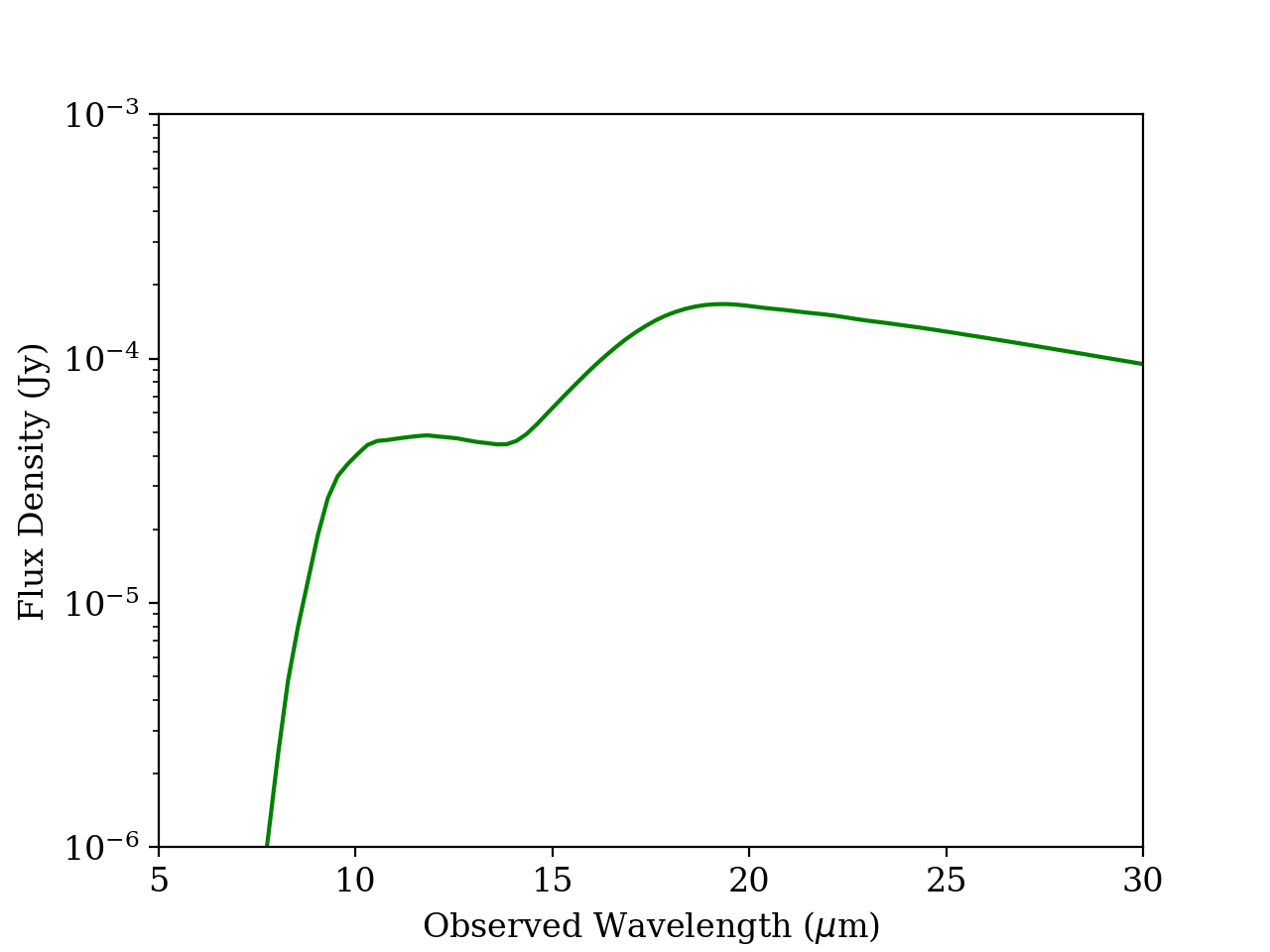
Silicate dust model. Simple example of a silicate SED model created with dustysn.
Fitting Data
In this page we will use SN2017eaw as an example using the data from Shahbandeh et al. 2023. First thing to do is to import the data, which has to be stored in a text file with a flux, flux error, upper limit, filter, telescope, and instrument columns in the format specified below. If no instrument or telescope is provided, the function will assume that the data is from JWST MIRI. The data must be structured as follows:
Flux |
Flux_err |
UL |
Filter |
Telescope |
Instrument |
|---|---|---|---|---|---|
6.39e-6 |
2.9e-7 |
False |
F560W |
JWST |
MIRI |
5.812e-5 |
7.9e-7 |
False |
F1000W |
JWST |
MIRI |
5.117e-5 |
1.25e-6 |
False |
F1130W |
JWST |
MIRI |
4.33e-5 |
5.8e-7 |
False |
F1280W |
JWST |
MIRI |
6.326e-5 |
6.9e-7 |
False |
F1500W |
JWST |
MIRI |
1.17e-4 |
1.28e-6 |
False |
F1800W |
JWST |
MIRI |
1.282e-4 |
1.61e-6 |
False |
F2100W |
JWST |
MIRI |
1.0247e-4 |
6.08e-6 |
False |
F2550W |
JWST |
MIRI |
The fit_dust_model is the main function used to fit the data, which uses MCMC to fit the dust emission model to the data.
from dustysn.model import import_data, fit_dust_model

# Define the parameters of the model
filename = 'SN2017eaw.txt' # File containing the data
object_name = 'SN2017eaw' # Name of the object
redshift = 0.001605 # Redshift of the object
composition = 'silicate' # Composition of the dust ('silicate' or 'carbon')
grain_size = 0.1 # Grain size in microns
n_components = 1 # Number of dust components to fit (1 or 2)

# Define the parameters of the fit
n_steps = 400 # Number of steps in the MCMC fit
n_walkers = 50 # Number of walkers in the MCMC fit
n_cores = 6 # Number of parallel cores to use for the fit
sigma_clip = 2 # Sigma clipping to remove outliers
repeats = 2 # Number of times to repeat the fit

# Import data
obs_wave, obs_flux, obs_flux_err, obs_limits, obs_filters, obs_wave_filters, obs_trans_filters = import_data('SN2017eaw.txt')

# Fit the model
results_1 = fit_dust_model(obs_wave, obs_flux, obs_flux_err, obs_limits, redshift, object_name,
                          composition=composition, grain_size=grain_size, n_components=n_components, n_walkers=n_walkers,
                          n_steps=n_steps, n_cores=n_cores, sigma_clip=sigma_clip, repeats=repeats,
                          obs_wave_filters=obs_wave_filters, obs_trans_filters=obs_trans_filters,
                          plot=True, output_dir='.', add_sigma=False)
Alternatively, if you want to specify a distance in addition to a redshift, you can do so by adding the distance parameter,
which must be an astropy.Quantity object with distance units (e.g., distance=10*u.Mpc). If you do not provide a distance,
this will be calculated from the redshift using the default cosmology in Astropy. Even if you specify a distance, you must
still provide a redshift, as this is used to calculate the rest-frame wavelengths.
from dustysn.model import import_data, fit_dust_model

# Define the parameters of the model
filename = 'SN2017eaw.txt' # File containing the data
object_name = 'SN2017eaw' # Name of the object
redshift = 0.001605 # Redshift of the object
distance = 7.12 * u.Mpc # Distance to the object
composition = 'silicate' # Composition of the dust ('silicate' or 'carbon')
grain_size = 0.1 # Grain size in microns
n_components = 1 # Number of dust components to fit (1 or 2)

# Define the parameters of the fit
n_steps = 400 # Number of steps in the MCMC fit
n_walkers = 50 # Number of walkers in the MCMC fit
n_cores = 6 # Number of parallel cores to use for the fit
sigma_clip = 2 # Sigma clipping to remove outliers
repeats = 2 # Number of times to repeat the fit

# Import data
obs_wave, obs_flux, obs_flux_err, obs_limits, obs_filters, obs_wave_filters, obs_trans_filters = import_data('SN2017eaw.txt')

# Fit the model
results_1 = fit_dust_model(obs_wave, obs_flux, obs_flux_err, obs_limits, redshift, object_name,
                          composition=composition, grain_size=grain_size, n_components=n_components, n_walkers=n_walkers,
                          n_steps=n_steps, n_cores=n_cores, sigma_clip=sigma_clip, repeats=repeats,
                          obs_wave_filters=obs_wave_filters, obs_trans_filters=obs_trans_filters,
                          plot=True, output_dir='.', add_sigma=False, distance=distance)
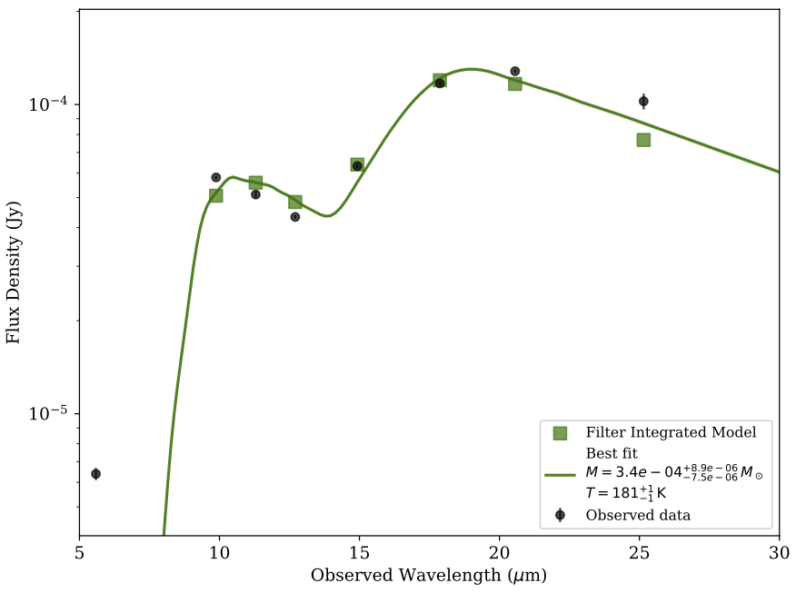
One Component Model Fit. Example of a one component model fit to the data of SN2017eaw, without additional variance.
As you can see there are a couple of problems with this model. First, the single dust model does not accurately fit the bluest data point.
Second, the model appears very tightly constrained with very small error bars, which is not realistic. To solve the second problem we can introduce
and additional variance to the model by setting the add_sigma parameter to True in the fit_dust_model function. This parameter will account
for an underestimation of the flux errors.
# Import data
obs_wave, obs_flux, obs_flux_err, obs_limits, obs_filters, obs_wave_filters, obs_trans_filters = import_data('SN2017eaw.txt')

# Fit the model
results_1 = fit_dust_model(obs_wave, obs_flux, obs_flux_err, obs_limits, redshift, object_name,
                          composition=composition, grain_size=grain_size, n_components=n_components, n_walkers=n_walkers,
                          n_steps=n_steps, n_cores=n_cores, sigma_clip=sigma_clip, repeats=repeats,
                          obs_wave_filters=obs_wave_filters, obs_trans_filters=obs_trans_filters,
                          plot=True, output_dir='.', add_sigma=True)
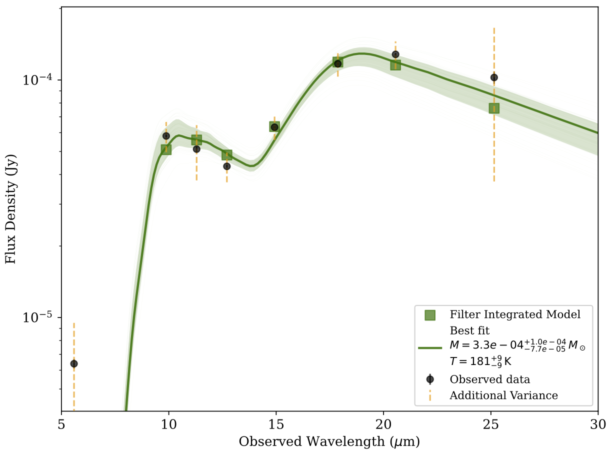
One Component Model Fit. Example of a one component model fit to the data of SN2017eaw, with additional variance sigma denoted by the orange dashed lines.
Now the model spread is more realistic. The emcee package in dustysn takes in a few parameters to run which depend on your specific system. The first are
the number of steps and walkers n_steps and n_walkers, the higher the number the more likely the model will converge to a good fit, but it will also take longer to run.
dustysn then takes an additional sigma_clip and repeats parameters, which are used to remove outliers from the data and repeat the fit multiple times to speed up convergence.
Below we show an example of a trace plot of the MCMC fit, which shows the evolution of the parameters during the fit. Additionally, the plot reports the R-hat statistic, which is a measure of convergence of the MCMC chains.
This is called the Gelman-Rubin statistic, and it should be close to 1 for a well-converged chain. If it is significantly larger than 1, it indicates that the chains have not converged yet.
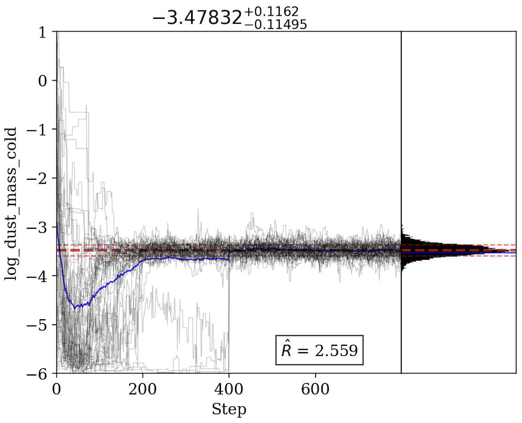
Trace Plot for cold dust mass. Example of a trace plot for the cold dust mass parameter during the MCMC fit with repeats=2. It is clear from the figure that mid way through the fit, the chains get re-sampled.
Now that we have addressed the error bar problem, we are still left with the problem of the model not fitting the bluest data point. To solve this we will add an additional dust component to the model.
To do this, we can simply change the n_components parameter to 2 in the fit_dust_model function. You can specify different compositions for the hot and cold dust components, using the
composition_hot and composition_cold parameters, respectively. For now, grain size must be the same for both components, but you can change it in the grain_size parameter.
from dustysn.model import import_data, fit_dust_model

# Define the parameters of the model
filename = 'SN2017eaw.txt' # File containing the data
object_name = 'SN2017eaw' # Name of the object
redshift = 0.001605 # Redshift of the object
composition = 'silicate' # Composition of the dust ('silicate' or 'carbon')
grain_size = 0.1 # Grain size in microns
n_components = 2 # Number of dust components to fit (1 or 2)

# Define the parameters of the fit
n_steps = 600 # Number of steps in the MCMC fit
n_walkers = 50 # Number of walkers in the MCMC fit
n_cores = 6 # Number of parallel cores to use for the fit
sigma_clip = 2 # Sigma clipping to remove outliers
repeats = 3 # Number of times to repeat the fit

# Import data
obs_wave, obs_flux, obs_flux_err, obs_limits, obs_filters, obs_wave_filters, obs_trans_filters = import_data('SN2017eaw.txt')

# Fit the model
results_1 = fit_dust_model(obs_wave, obs_flux, obs_flux_err, obs_limits, redshift, object_name,
                          composition_hot=composition, composition_cold=composition, grain_size=grain_size,
                          n_components=n_components, n_walkers=n_walkers,
                          n_steps=n_steps, n_cores=n_cores, sigma_clip=sigma_clip, repeats=repeats,
                          obs_wave_filters=obs_wave_filters, obs_trans_filters=obs_trans_filters,
                          plot=True, output_dir='.', add_sigma=True)
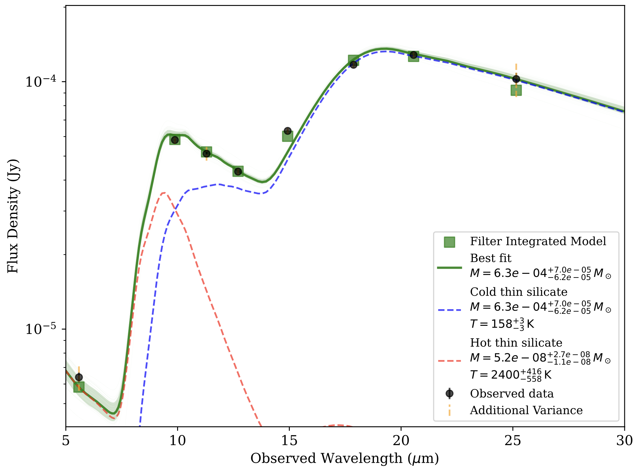
Two Component Model Fit. Example of a model fit using a two component model to the data of SN2017eaw.
The code will also save a corner plot that can allow you to visualize the posterior distributions of the parameters and explore the correlations between them. This is useful to understand the uncertainties in the model parameters.
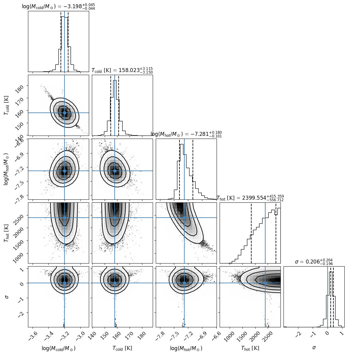
Corner Plot for Two Component Model Fit. Example of a corner plot for the two component model fit to the data of SN2017eaw.
In this case it is also evident that the temperature of the hot dust component is not well constrained, but is instead hitting the prior of 3000K, which is chosen based on the photodissociation temperature of the dust. This means that the temperature of the hot component could be much higher, but that our data is not able to constrain it.
That is a better fit to the data, but how do we know that? The full_model function also generates a comparsion plot in which it compares the one component
fit and the two component fit to the data, as well as the BIC and AIC values for both models. The BIC (Bayesian Information Criterion) and AIC (Akaike Information Criterion)
are both used to penalize models for their complexity, with lower values indicating a better fit.
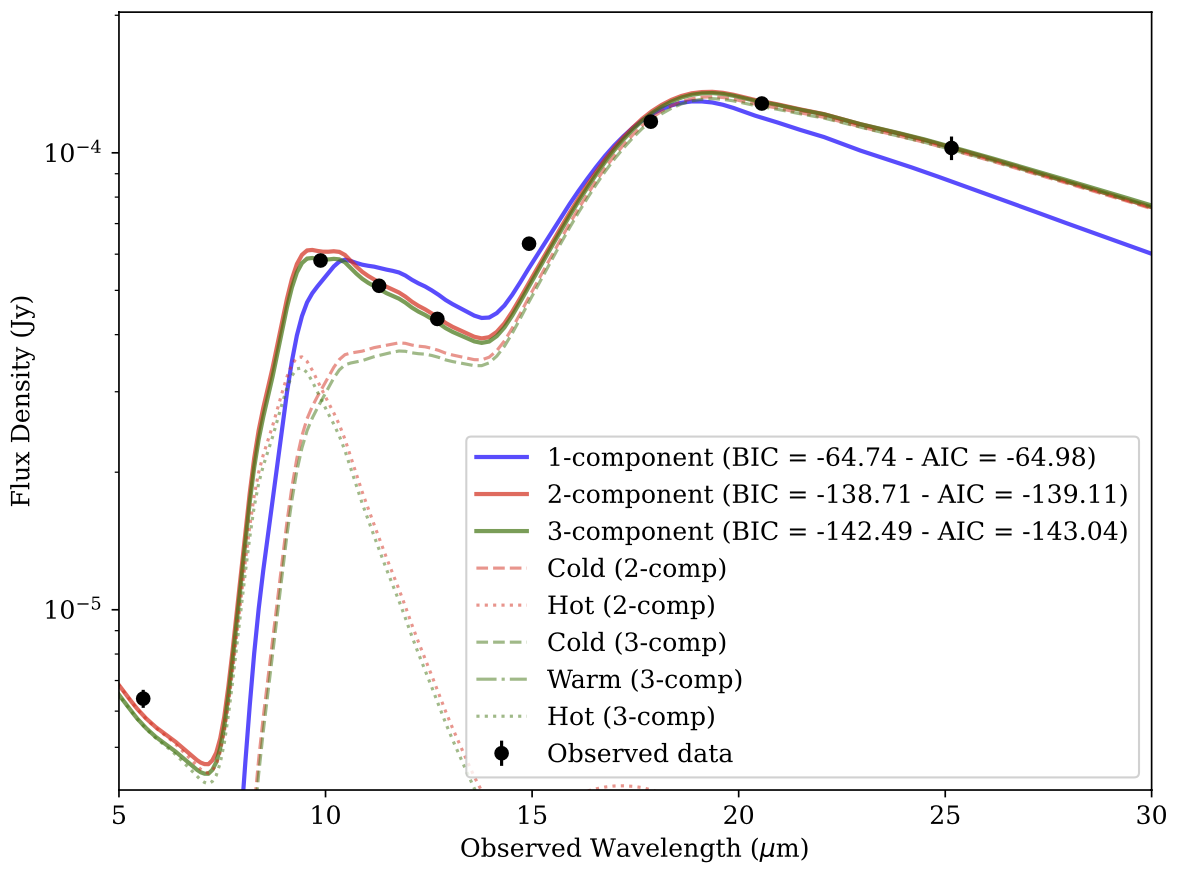
BIC and AIC Comparison. Example of a BIC and AIC comparison between the one, two, and three component model fit to the data of SN2017eaw.
In this case, the two component model is preferred over the one component model. Make sure to compare the difference between the BIC and AIC values, as the absolute values depend on the number of data points and the number of parameters in the model. In this case the two component model is significantly lower than the one component model, indicating that it is a better fit to the data. The three component model is only marginally better than the two component model, but it is probably not worth the additional complexity.
Optically Thick Case
You can also choose to fit optically thick dust by specifying dust_type = 'thick'. In this case you must also
specify the radius of the dust shell in cm using the radius parameter. All the other parameters and functionality
are the same as before.